基本的采样方法

概述

本文介绍一些基本的采样方法.

均匀分布的采样

均匀分布的样本产生方法核心为在计算机中生成[0,1]之间的伪随机数序列,该序列可以用于[0,1]之间均匀分布的样本

伪随机数的产生最简单的方法为线性同余法. 它是根据递归公式： $N_{j+1} = (A * N_{j} + B) \quad mod \quad M$

LCG的周期最大为M，但大部分情况都会少于M。要令LCG达到最大周期，应符合以下条件：

B,M互质；
M的所有质因数都能整除 A-1；
若 M是4的倍数， A-1也是；
$A,B,N_{0}$ 都比M小；
A,B是正整数。

在Python random包中random的伪随机产生是用c写的,代码如下

/* generates a random number on [0,0xffffffff]-interval */
static unsigned long
genrand_int32(RandomObject *self)
{
    unsigned long y;
    static unsigned long mag01[2]={0x0UL, MATRIX_A};
    /* mag01[x] = x * MATRIX_A  for x=0,1 */
    unsigned long *mt;

    mt = self->state;
    if (self->index >= N) { /* generate N words at one time */
        int kk;

        for (kk=0;kk<N-M;kk++) {
            y = (mt[kk]&UPPER_MASK)|(mt[kk+1]&LOWER_MASK);
            mt[kk] = mt[kk+M] ^ (y >> 1) ^ mag01[y & 0x1UL];
        }
        for (;kk<N-1;kk++) {
            y = (mt[kk]&UPPER_MASK)|(mt[kk+1]&LOWER_MASK);
            mt[kk] = mt[kk+(M-N)] ^ (y >> 1) ^ mag01[y & 0x1UL];
        }
        y = (mt[N-1]&UPPER_MASK)|(mt[0]&LOWER_MASK);
        mt[N-1] = mt[M-1] ^ (y >> 1) ^ mag01[y & 0x1UL];

        self->index = 0;
    }

    y = mt[self->index++];
    y ^= (y >> 11);
    y ^= (y << 7) & 0x9d2c5680UL;
    y ^= (y << 15) & 0xefc60000UL;
    y ^= (y >> 18);
    return y;
}

/* random_random is the function named genrand_res53 in the original code;
 * generates a random number on [0,1) with 53-bit resolution; note that
 * 9007199254740992 == 2**53; I assume they're spelling "/2**53" as
 * multiply-by-reciprocal in the (likely vain) hope that the compiler will
 * optimize the division away at compile-time.  67108864 is 2**26.  In
 * effect, a contains 27 random bits shifted left 26, and b fills in the
 * lower 26 bits of the 53-bit numerator.
 * The orginal code credited Isaku Wada for this algorithm, 2002/01/09.
 */
static PyObject *
random_random(RandomObject *self)
{
    unsigned long a=genrand_int32(self)>>5, b=genrand_int32(self)>>6;
    return PyFloat_FromDouble((a*67108864.0+b)*(1.0/9007199254740992.0));
}

在Python random库中也提供Wichman-Hill伪随机数生成器

class WichmannHill(Random):
  def random(self):
    """Get the next random number in the range [0.0, 1.0)."""

    # Wichman-Hill random number generator.
    #
    # Wichmann, B. A. & Hill, I. D. (1982)
    # Algorithm AS 183:
    # An efficient and portable pseudo-random number generator
    # Applied Statistics 31 (1982) 188-190
    #
    # see also:
    #        Correction to Algorithm AS 183
    #        Applied Statistics 33 (1984) 123
    #
    #        McLeod, A. I. (1985)
    #        A remark on Algorithm AS 183
    #        Applied Statistics 34 (1985),198-200

    # This part is thread-unsafe:
    # BEGIN CRITICAL SECTION
    x, y, z = self._seed
    x = (171 * x) % 30269
    y = (172 * y) % 30307
    z = (170 * z) % 30323
    self._seed = x, y, z
    # END CRITICAL SECTION

    # Note:  on a platform using IEEE-754 double arithmetic, this can
    # never return 0.0 (asserted by Tim; proof too long for a comment).
    return (x/30269.0 + y/30307.0 + z/30323.0) % 1.0

常见分布的直接采样方法

直接采样方法, Inverse CDF

离散随机变量的例子

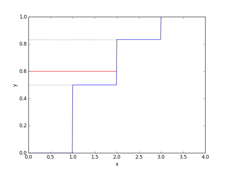
设一个离散随机变量x,可以取值(1,2,3), 不同取值的概率分别为$(\frac{1}{2},\frac{1}{3},\frac{1}{6})$, 要生成变量x的样本,样本的分布服从上述pmf,直接的做法为,

从[0,1)区间用均匀分布产生随机样本y
若y<1/2，则对应输出x=1的一个样本, 若1/2<y<(1/2+1/3)，则对应输出x=2的一个样本, 若(1/2+1/3)<y，则对应输出x=3的一个样本.

上述方法简单,并且很容易理解. 实际上就是对随机变量X的cdf求逆的过程, 从[0,1)区间用均匀分布产生随机样本y,然后根据随机变量x的cdf找到对应的x的值.

为了更直观的看清楚问题,我们将x变量分布的cdf画出来

discrete_cdf

import matplotlib.pyplot as plt
import numpy as np

def calc_cdf(x):
    if x < 1.0:
        return 0.0
    if 1.0 <= x < 2.0:
        return 1.0/2.0
    if 2.0 <= x < 3.0:
        return 1.0/2.0 + 1.0/3.0
    if 3.0 <= x:
        return 1.0

# generate 100 points
M=100
x=map(lambda x: x/float(M),range(0,M*4))
y = map(calc_cdf, x)

# plot cdf
plt.plot(x,y)

# plot line
x1 = filter(lambda x: x<1.0, x)
y1 = (np.ones(len(x1)) * 0.5).tolist()
plt.plot(x1,y1,color='g',ls='dotted')

x2 = filter(lambda x: x < 2.0, x)
y2 = (np.ones(len(x2)) * (1.0/2.0 + 1.0/3.0)).tolist()
plt.plot(x2,y2,color='g',ls='dotted')

x3 = filter(lambda x: x < 2.0, x)
y3 = (np.ones(len(x3)) * 0.6).tolist()
plt.plot(x3,y3,color='r')

plt.ylabel('y')
plt.xlabel('x')

plt.show()

连续随机变量的例子

原理同离散随机变量, 从均匀分布产生随机值y,由y值,根据cdf曲线找到对应的x的值, 该x的值为产生的随机样本.

以指数分布为例,其cdf如下

$y = 1 - e^{-\lambda x}$

其cdf的逆函数为

$e^{-\lambda x} = 1 - y$ $-\lambda x = ln(1 - y)$ $x = -\frac{ln(1 - y)}{\lambda}$

贴一张wiki上的图片做说明

exp_cdf

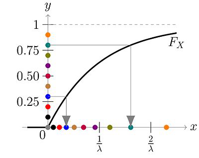
注,在cdf的逆函数中，如果用y代替1-y,其分布是不会改变的. 因为y是在[0,1)区间上的均匀分布. 所以在实际实现中是用y来取代1-y. 也就是 $- \frac{ln(y)}{\lambda}$

下面是python random包中关于产生服从指数分布的随机样本的代码

def expovariate(self, lambd):
       """Exponential distribution.

       lambd is 1.0 divided by the desired mean.  It should be
       nonzero.  (The parameter would be called "lambda", but that is
       a reserved word in Python.)  Returned values range from 0 to
       positive infinity if lambd is positive, and from negative
       infinity to 0 if lambd is negative.

       """
       # lambd: rate lambd = 1/mean
       # ('lambda' is a Python reserved word)

       random = self.random
       u = random()
       while u <= 1e-7:
           u = random()
       return -_log(u)/lambd

使用Inverse CDF来做采样有个限制条件,就是需要找到对应随机分布的CDF的解析表达,以及其逆函数的解析表达. 否则计算上比较麻烦.

非常重要的一个分布,高斯分布的CDF就没有解析表达. 高斯分布的CDF, $\Phi (x)={\frac {1}{\sqrt {2\pi }}}\int_{-\infty}^{x} e^{-t^{2}/2} dt$

高斯分布的box-muller变换方法

当变量x和y为区间[0, 1)上均匀分布的独立变时, 使用下列变换得到变量$Z_0, Z_1$,

$Z_0 = cos(2*\pi*x) * \sqrt{-2*log(1-y)}$ $Z_1 = sin(2*\pi*x) * \sqrt{-2*log(1-y)}$

变量$Z_0,Z_1$ 为两个服从均值为0,方差为1的独立高斯分布随机变量

python random包中高斯分布样本生成的代码如下

def gauss(self, mu, sigma):

        random = self.random
        z = self.gauss_next
        self.gauss_next = None
        if z is None:
            x2pi = random() * TWOPI
            g2rad = _sqrt(-2.0 * _log(1.0 - random()))
            z = _cos(x2pi) * g2rad
            self.gauss_next = _sin(x2pi) * g2rad

        return mu + z*sigma

参考

https://en.wikipedia.org/wiki/Inverse_transform_sampling